
Cross Entropy Loss Connection to GPT Models
Most applied researchers or ml engineers use F.cross_entropy(logits, labels) dozens of times a week. But, not a lot of them could explain, from first principles, why that particular function is the right one to minimize.
The answer turns out to be both simpler and deeper than most people expect. It starts with a coin and ends with GPT-5 (as of today).
Table of Contents
- What Is Maximum Likelihood Estimation?
- The Log Trick: Why Log-Likelihood Is Numerically Stable
- The Sign Flip: Connecting MLE to Gradient Descent
- Binary Cross-Entropy Loss Is Exactly NLL
- Why the Cross-Entropy Gradient Self-Adjusts (and MSE Doesn’t)
- How LLM Training Loss and Perplexity Are Just MLE at Scale
- RLHF, VAEs, and Diffusion Models: MLE in Disguise
- Summary
What Is Maximum Likelihood Estimation?
You flip a fair-ish coin 10 times. You get 7 heads and 3 tails. What is your best estimate for the coin’s probability of heads?
Your gut says 0.7. You are right. But here is the uncomfortable question: why exactly 0.7? Why not 0.71? Why not 0.68, which would “hedge” toward 0.5 to account for sampling noise?
There is a precise, mathematical reason 0.7 is the correct answer, and understanding that reason is the same as understanding why every modern neural network trains the way it does.
The key move is to stop thinking about probability the way most people do. Normally, you fix the parameters (the coin bias) and ask how probable a particular outcome is. MLE inverts this.
You fix the data: the seven heads and three tails you already observed and ask which parameter value makes that specific data most probable. You treat the data as a constant and turn the parameter into a variable.
The function you are now maximizing over is called the likelihood function:
\[L(\theta) = \theta^7 \cdot (1-\theta)^3\]This is the probability of seeing exactly seven heads and three tails, as a function of the coin’s bias theta. It is not a probability distribution over theta, it does not integrate to one, and it has no obligation to. It is just a lens that lets you ask: “For which value of theta was this particular dataset most probable?”
Here’s a code snippet which sweeps theta from 0 to 1 and evaluates the likelihood at each point:
import numpy as np

theta = np.linspace(0.001, 0.999, 1000)
n_heads, n_tails = 7, 3
N = n_heads + n_tails

likelihood = theta**n_heads * (1 - theta)**n_tails
theta_mle = n_heads / N   # = 0.7
As shown below, a smooth curve peaking at theta = 0.7.
The peak is the MLE estimate. Taking the derivative and setting it to zero gives theta-hat = 7/10 = 0.7 analytically. MLE formalizes the intuition your gut already had.
The calculus is clean. Differentiate L(theta), set to zero, and you get:
\[7(1-\theta) = 3\theta \implies 7 = 10\theta \implies \hat{\theta} = 0.7\]So MLE is not an approximation or a heuristic. It is the exact answer to a precise question: “Given this data, what is the most plausible parameter value?”
The Log Trick: Why Log-Likelihood Is Numerically Stable
So far so good. But here is the problem: real datasets are not ten coin flips. They are ten million data points, each contributing one multiplicative factor to the likelihood. A product of a million numbers, each between zero and one, is so astronomically small that any computer will immediately round it to zero. You cannot even represent it in float64.
And even if you could, products are miserable to differentiate. Every application of the product rule adds terms.
The solution is the log trick, and it is elegant.
The logarithm is a monotonically increasing function, which means it preserves the location of maxima. The theta that maximizes L(theta) is identical to the theta that maximizes log L(theta). They have the same peak, just a different y-axis.
But log does something transformative to the structure of the function. Products become sums:
\[\log L(\theta) = \log(\theta^7 \cdot (1-\theta)^3) = 7 \log \theta + 3 \log(1-\theta)\]And in general, for N independent observations:
\[\log L(\theta) = \sum_{i=1}^{N} \log P(x_i \mid \theta)\]So a product of a million tiny numbers becomes a sum of a million negative numbers. Numerically stable. Easy to differentiate term by term.
What this does: Computes the log-likelihood, a sum instead of a product.
log_likelihood = n_heads * np.log(theta) + n_tails * np.log(1 - theta)
As shown below, a concave curve, also peaking at theta = 0.7, but now ranging from around -7 to 0 rather than 0 to 0.00023.
The peak is at the same theta. The log trick is a free lunch, same answer, much better numerics, much simpler derivatives.
The shape changes (it is now concave rather than the asymmetric hump of the original), but the fundamental question, where is the maximum has the same answer. This is the log trick. It is used everywhere in statistics and machine learning, often without comment, as if it is so obvious it barely deserves naming.
The Sign Flip: Connecting MLE to Gradient Descent
Here is the bridge. Gradient descent minimizes functions. MLE maximizes likelihood. So there is a direction mismatch. The fix requires exactly one operation: flip the sign.
\[\arg\max_\theta \log L(\theta) \quad = \quad \arg\min_\theta \underbrace{-\log L(\theta)}_{\text{Negative Log-Likelihood (NLL)}}\]That is it. That is the entire bridge between maximum likelihood estimation and gradient descent. You negate the log-likelihood, call the result negative log-likelihood and now gradient descent can minimize it while doing exactly what MLE would have done.
The code below flips the log-likelihood to get NLL, a function we can minimize.
nll = -log_likelihood
# nll.argmin() gives the same index as log_likelihood.argmax()
print(f"MLE theta: {theta[nll.argmin()]:.3f}")   # 0.700
As shown below, a convex curve (U-shaped), with its minimum at theta = 0.7.
In Pytorch, every time you call .backward() on a cross-entropy loss in PyTorch, you are computing gradients of NLL, and those gradients are pushing your parameters toward the MLE solution.
So when someone says we trained this model with cross-entropy loss, what they are actually saying is we found the maximum likelihood estimate of the model’s parameters given the training data. The two statements are mathematically identical. One is the statistician’s phrasing, the other is the ML engineer’s phrasing.
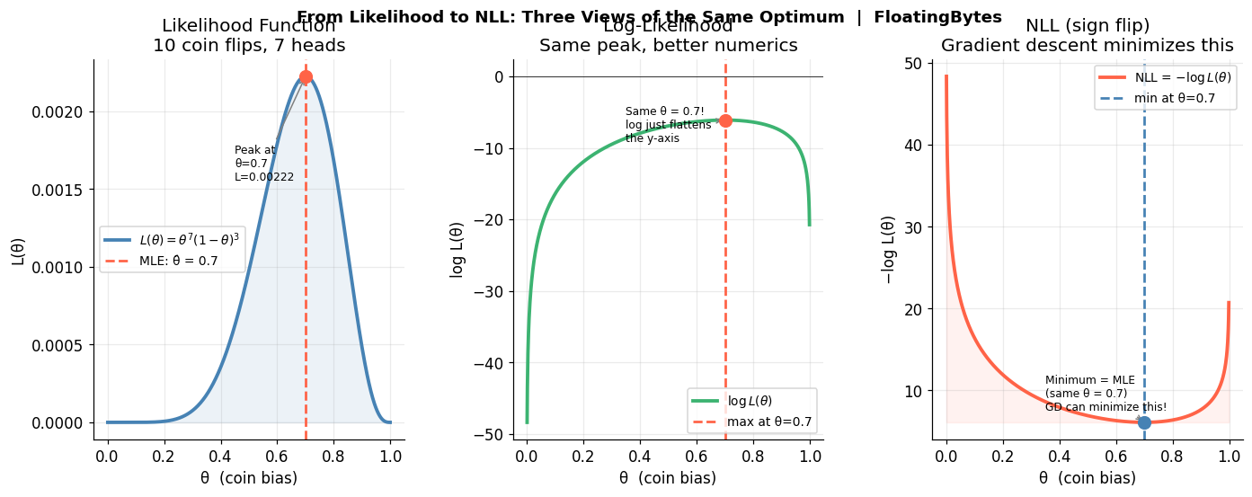 Three views of the same optimum: likelihood L(θ), log-likelihood log L(θ), and NLL −log L(θ) all locate their peak or minimum at θ = 0.7.
Binary Cross-Entropy Loss Is Exactly NLL
Now apply this to a binary classifier. The model takes in some features and outputs a single number, which a sigmoid squashes to a probability p-hat between 0 and 1. You want p-hat close to 1 when the true label is 1, and close to 0 when the true label is 0.
The probability the model assigns to the observed label y (which is either 0 or 1) is:
\[P(y \mid \hat{p}) = \hat{p}^y \cdot (1-\hat{p})^{1-y}\]Check this for yourself. If y = 1, this collapses to p-hat. If y = 0, this collapses to (1 - p-hat). This is the Bernoulli probability mass function, with p-hat as the parameter.
Take the negative log of this, average over N examples, and you get:
\[\mathcal{L}_{BCE} = -\frac{1}{N}\sum_{i=1}^N \left[ y_i \log \hat{p}_i + (1-y_i)\log(1-\hat{p}_i) \right]\]That formula is binary cross-entropy loss. And it is not approximately equal to the NLL of a Bernoulli model. It is not inspired by the NLL of a Bernoulli model. It is the NLL of a Bernoulli model. Exactly, directly, completely.
The code below evaluates binary cross-entropy for positive and negative examples:
p_hat = np.linspace(0.001, 0.999, 1000)

bce_positive = -np.log(p_hat)        # y=1: loss when true label is positive
bce_negative = -np.log(1 - p_hat)    # y=0: loss when true label is negative
Lets focus on the two curves below. For y=1, loss is high when p-hat is low (model is wrong) and approaches zero as p-hat approaches one. For y=0, the mirror image.
The asymmetry is not a design choice. It follows directly from the log of a Bernoulli probability. Being confidently wrong produces enormous loss because log of a near-zero probability is a large negative number, and we are minimizing the negation.
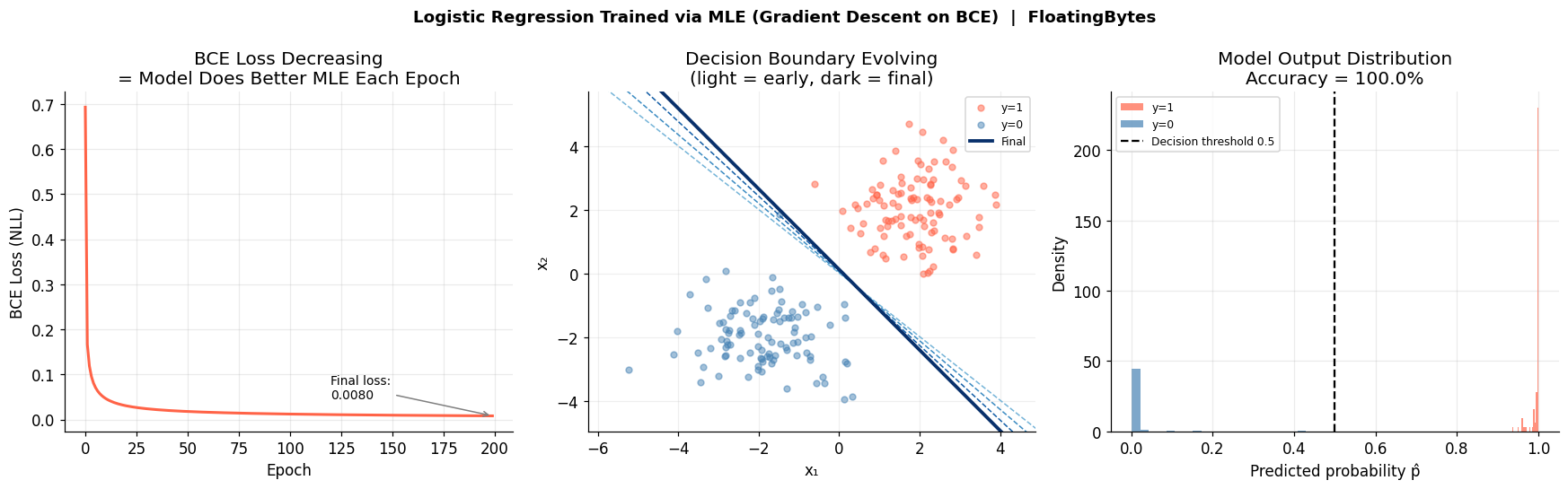 Left: BCE loss decreasing over 200 epochs. Center: decision boundary rotating into place (light = early, dark = final). Right: model output distribution separating cleanly after training.
The loss when p-hat = 0.001 and y = 1 is -log(0.001) = 6.9. When p-hat = 0.999 and y = 1, it is -log(0.999) = 0.001. The model is not penalized lightly for being confidently wrong. It is penalized in a way that grows without bound as the predicted probability approaches zero.
Why the Cross-Entropy Gradient Self-Adjusts (and MSE Doesn’t)
One of the most underappreciated properties of log loss is what happens to its gradient. The derivative of -log(p) with respect to p is -1/p. Think about what that means.
When the model assigns a probability of 0.9 to the correct class, the gradient magnitude is 1/0.9 = 1.1. Small. The model is already doing well; the update should be gentle.
When the model assigns a probability of 0.1 to the correct class, the gradient magnitude is 1/0.1 = 10. Ten times larger. The model is very wrong; it deserves a forceful correction.
When the model assigns a probability of 0.001, the gradient is 1000. The model is catastrophically miscalibrated; the update is proportionally aggressive.
This self-adjusting behavior is not a feature that was engineered in. It emerges directly from the shape of the logarithm. The log curve is steep near zero and flat near one and since we are minimizing its negation, that translates into large gradients when the model is wrong and small gradients when it is right.
The code below computes and plots gradient magnitude as a function of predicted probability.
p = np.linspace(0.001, 0.999, 2000)
neg_log_p = -np.log(p)
grad_magnitude = 1 / p    # derivative of -log(p) w.r.t. p is -1/p, magnitude is 1/p
Below we see a hyperbola decreasing from very large values near p=0 to approaching 1 near p=1.
Compare to MSE, the gradient of (1-p)^2 is 2(1-p), which is at most 2 (when p=0). BCE gradients are unbounded as p approaches zero. This is why BCE trains classification models dramatically faster than MSE the loss function is essentially shrieking at the model when it makes confident mistakes.
The difference is stark in practice. At p-hat = 0.01 with a true label of 1:
- BCE loss = -log(0.01) = 4.60, gradient = 100
- MSE loss = (1 - 0.01)^2 = 0.98, gradient = 1.98
MSE is capped. BCE is not. BCE keeps screaming at the model until it gets the probability right.
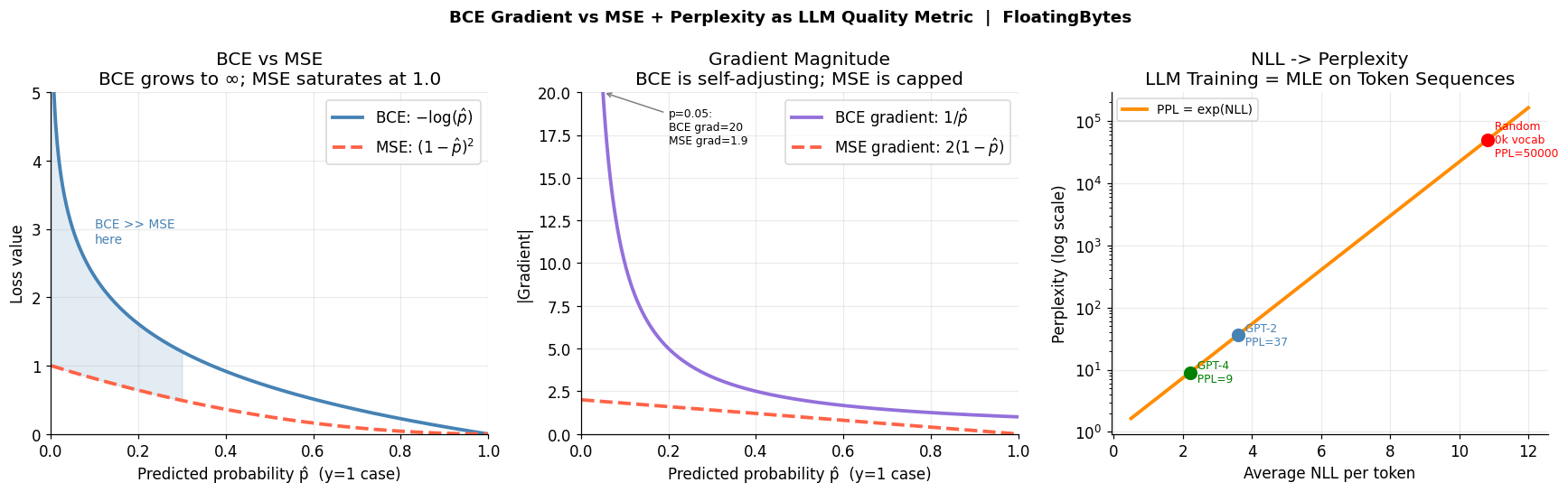 Left: BCE grows to infinity as p̂ → 0; MSE caps at 1.0. Center: gradient magnitude 1/p vs the bounded MSE gradient. Right: the exponential NLL → perplexity curve, with GPT-2 and GPT-4 marked.
How LLM Training Loss and Perplexity Are Just MLE at Scale
Everything above scales directly to large language models, and the translation is surprisingly literal.
A language model is trained on text sequences. Each sequence is a list of tokens: words, subwords, punctuation marks. The model’s job is to predict the next token given all previous tokens. At each position t, the model outputs a probability distribution over the entire vocabulary, maybe 50,000 tokens using a softmax layer.
The probability the model assigns to the entire sequence is the product of its per-token predictions:
\[P(w_1, w_2, \ldots, w_T) = \prod_{t=1}^{T} P(w_t \mid w_1, \ldots, w_{t-1})\]Take the negative log, average over all T positions, and you get the training loss:
\[\mathcal{L} = -\frac{1}{T}\sum_{t=1}^{T} \log P(w_t \mid w_1, \ldots, w_{t-1})\]And this is exactly what CrossEntropyLoss computes over the vocabulary at each token position. LLM training is MLE. Maximum likelihood estimation of the parameters of the model, given the training corpus as observed data.
What this does: Simulates per-token NLL for models of different quality and converts to perplexity.
models = {
    'Random (no learning)':  {'mean_nll': np.log(50_000)},   # log(50000) ≈ 10.8
    'GPT-2 (117M)':          {'mean_nll': 3.6},
    'GPT-4 class (est.)':    {'mean_nll': 2.2},
}
perplexities = {k: np.exp(v['mean_nll']) for k, v in models.items()}
print(perplexities)
{'Random': 50000, 'GPT-2': 36.6, 'GPT-4': 9.0}
Perplexity = exp(NLL per token). A perplexity of 9 means the model is about as uncertain as if it were choosing uniformly among 9 options. A random guesser over a 50,000 word vocabulary has perplexity 50,000. The entire history of LLM progress is a story of driving this number down.
So when researchers compare GPT-2 to GPT-5, they are comparing two MLE solutions to the same problem, maximizing the likelihood of English text obtained with different model sizes and different amounts of compute. GPT-5’s lower perplexity means it found a better maximum-likelihood estimate of how language works.
The Cross-Entropy Loss Pipeline: From Coin Flip to GPT
(7H 3T coin flips)"] --> B["Likelihood
L(θ) = θ⁷(1-θ)³"] B --> C["Log-Likelihood
log L(θ) = 7logθ + 3log(1-θ)
product → sum"] C --> D["Negate
× -1
(sign flip)"] D --> E["NLL
-log L(θ)
Gradient descent minimizes"] E --> F1["Binary CE
-[y log p̂ + (1-y)log(1-p̂)]
Logistic regression"] E --> F2["Multi-class CE
-log p_true_class
after softmax"] E --> F3["LLM Loss
-(1/T)Σ log P(wₜ|ctx)
GPT, LLaMA, Gemini"] F3 --> G["Perplexity
exp(NLL per token)
GPT-2≈37, GPT-4≈9"]
RLHF, VAEs, and Diffusion Models: MLE in Disguise
Here is where it gets strange. The story does not end with classification and language modeling. It turns out that virtually every loss function in modern deep learning is, with some algebraic work, the NLL of some probability distribution under some modeling assumption.
Reinforcement Learning from Human Feedback (RLHF), the technique that makes ChatGPT follow instructions, trains a reward model using a loss that is -log(sigmoid(r_chosen - r_rejected)). That is the NLL of a Bradley-Terry pairwise preference model. MLE in disguise.
Variational Autoencoders minimize the Evidence Lower Bound (ELBO), which is a reconstruction term (NLL under Gaussian or Bernoulli assumptions) plus a KL divergence regularizer. The reconstruction term is NLL. MLE in disguise.
Even things that do not look like NLL at first, hinge loss, focal loss, contrastive loss, can often be interpreted as NLL under modified or reweighted likelihood models.
The entire modern AI training stack is, at its core, a coin-flip problem scaled to petabytes.
Summary
Cross-entropy loss is not a heuristic chosen because it works well empirically. It is the mathematically necessary result of asking the question “what parameters make my training data most probable?”
Answering that question gives you maximum likelihood estimation. Taking the log of the likelihood converts the product to a sum and makes derivatives tractable. Flipping the sign converts the maximization problem to a minimization problem that gradient descent can solve.
Did you find this post useful? I am curious to hear from you in comments below.

Comments