
Deep Dive into Fine Tuning a LoRA Reranker on Phi-3
I recently finished reading the huggingface playbook and got super excited about digging into the LLM internals.
So, I fine tuned a 3.8 billion parameter language model to rank search results and tried to visualise internals. Every gradient norm at every layer. Every attention pattern before and after. Every hidden state at five different depths of the network.
In this post, I want to share the behaviour of the phi 3 LLM on a reranking task using lora fine tuning on ms marco dataset.
Table of Contents
- The Coin Flip
- The Learning Phase
- Where the Gradients Went
- What about Attention layers
- The Ablation That Broke My Theory
- The Telescope
- Summary
Part 1: The Coin Flip
Basically, the dataset contains query -> relevant documents pairs. You give the language model a query and two documents and it tells you which document is more relevant. That’s it. Binary choice. “A or B?”
I took a real query from the MS MARCO passage ranking dataset like “what are the liberal arts?”, paired it with two passages (one relevant, one not), and formatted it like this:
Below is the prompt template I used.
RERANK_TEMPLATE = """Query: {query}

Document A: {doc_a}

Document B: {doc_b}

Which document is more relevant to the query? Answer A or B."""
As we know, the model generates hidden states for all vocab token. To get better visibility into the LLM learning, I take last token’s hidden state and project them to provide 2 logits: one for A, one for B. I think this is the simplest possible ranking formulation here. No listwise loss, no NDCG optimization. Just a coin flip that the model has to learn to make correctly. In this setup, we get two logits at the last layer which needs to be softmaxed later.
I used Phi-3 Mini model (3.8 billion parameters) and loaded in 4-bit quantization, with LoRA rank-16 adapters on the fused QKV projections. That’s 6.3 million trainable parameters out of 3.8 billion. 0.16%. Quite doable on A100 GPU machine.
Before starting training, I checked the baseline and the model’s eval accuracy was 53.5%. It’s almost like was flipping a coin. For our “liberal arts” query, it had absolutely no opinion about which passage was better.
Part 2: The Learning Phase
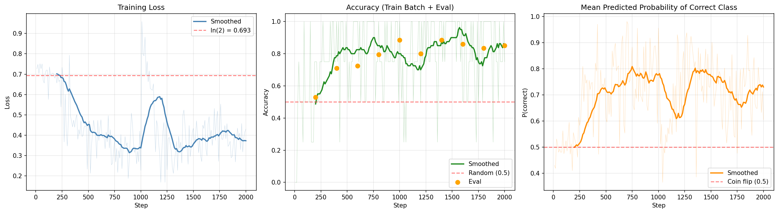
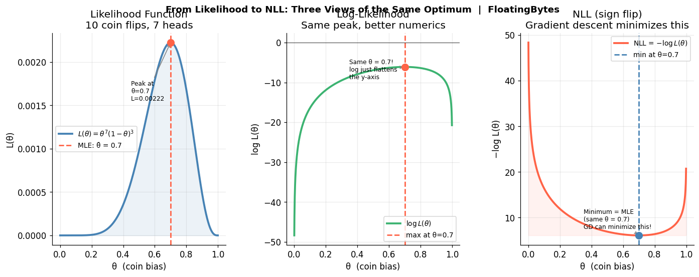
I expected the loss curve to go down gradually. Maybe a slow descent, maybe a plateau followed by steady improvement. What I got was a cliff.
For the first ~300 optimizer steps, the loss barely moved. It sat near $\ln(2) \approx 0.693$, the loss you get from predicting 50/50 on every input. The model was still coin flipping. At step 200, the eval accuracy was 53%. Indistinguishable from the untrained model. Then, somewhere around step 400, the accuracy jumped to 71%. By step 600 it was 72.5%. By step 1600 it hit 86%. I felt bit relieved.
The steepest drop in the smoothed loss happened at step ~1220, where the loss plunged from 0.57 to 0.34. In the span of a few hundred optimizer steps, the model went from “I have no idea” to “I’m right 87% of the time.”
I researched about this behaviour and found our that it has a name. It’s a phase transition, a discontinuous change in behavior where the model appears to be doing nothing and then suddenly reorganizes. You see this in grokking, in in-context learning emergence, and now apparently in LLM reranker fine-tuning.
Something was still missing, I thought: if the loss isn’t moving for 300 steps, the gradients aren’t zero, they’re flowing through the network every single step. What are they even DOING during that plateau? Is that all wasted compute?
Part 3: Where the Gradients Went
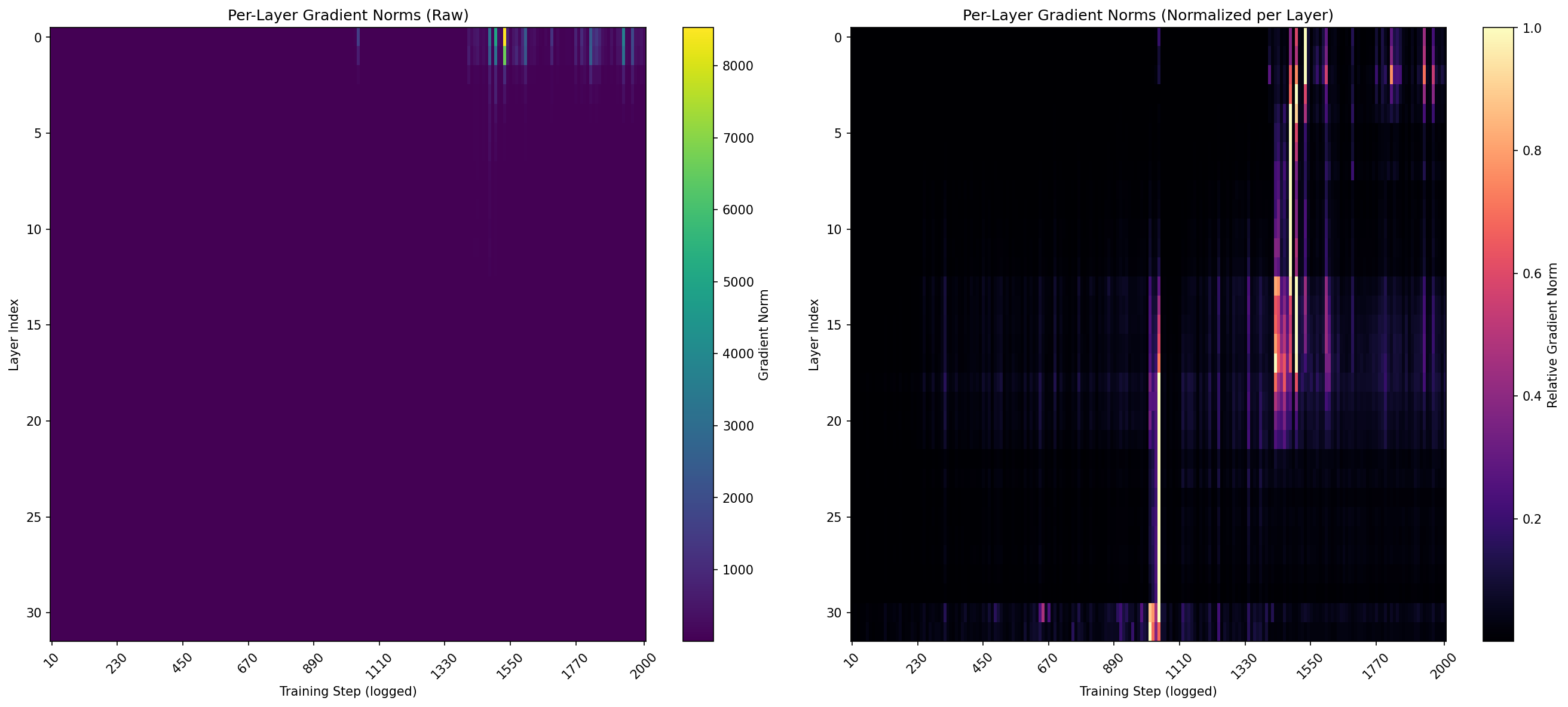
So I logged the gradient norms at every layer, at every optimizer step throughout training. This is the per-layer gradient norm $\sqrt{\sum g_i^2}$ for the LoRA parameters at each of the 32 transformer layers. It tells you how much each layer is being asked to change.
My hypothesis was straightforward: the late layers should dominate. They’re closest to the classification head, closest to the loss signal. The gradient has to backpropagate through fewer layers to reach them. And the ranking comparison “is A better than B?” feels like a high level reasoning task, which in transformer lore lives in the later layers.
I got it all wrong by a distance.
The code below shows the log the L2 norm of gradients for every LoRA adapter, grouped by layer. It provides a dict mapping each layer index to its mean gradient norm.
# Per-layer gradient norms (only for LoRA parameters)
layer_norms = defaultdict(list)
for name, param in model.named_parameters():
    if param.grad is not None and "lora" in name.lower():
        layer_idx = int(name.split("layers.")[1].split(".")[0])
        layer_norms[layer_idx].append(param.grad.norm().item())
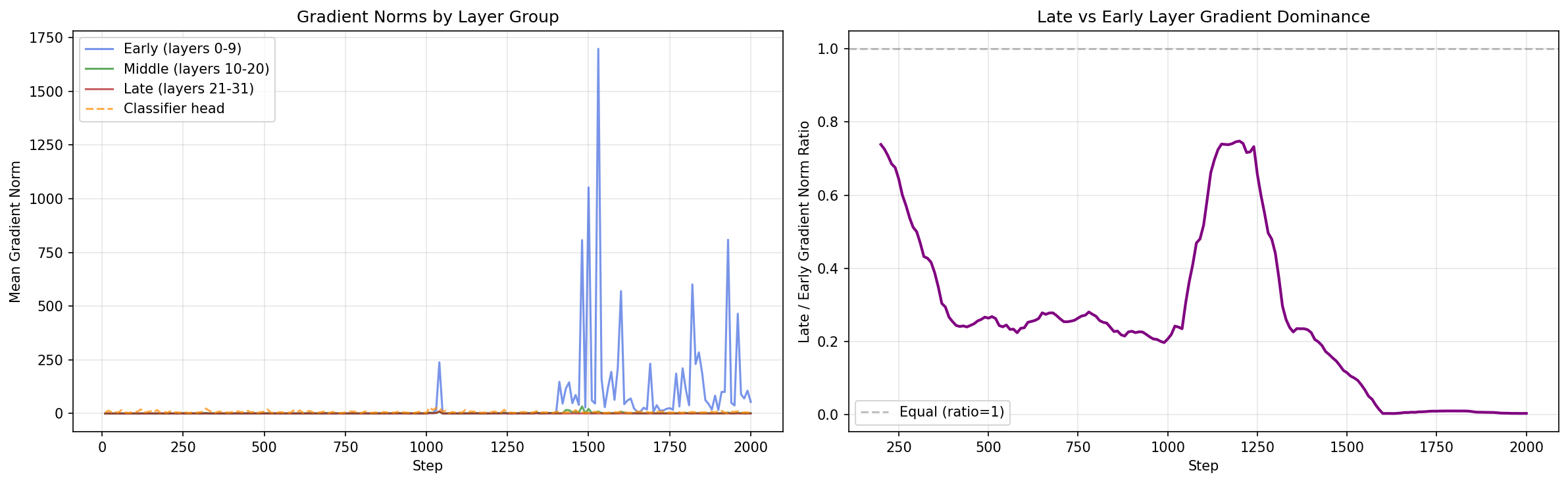
The numbers weren’t even close. Layer 0 had a mean gradient norm of 237. Layer 1: 196. Layer 2 dropped to 46. By layer 4 it was under 10. The late layers 21 through 31 with average 0.25.
Let me say that again in simple words. The first layer received 200 times more gradient signal than the last layer. Early layers (0-9) averaged 53.1. Middle layers (10-20) averaged 1.5. Late layers (21-31) averaged 0.25. The classifier head itself was at 6.6.
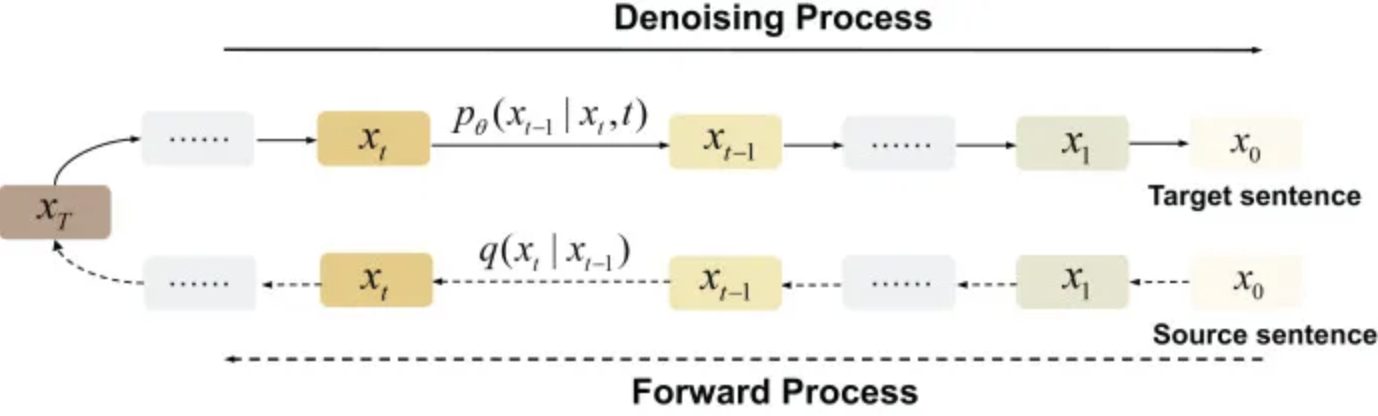
The gradient flows backward (left), but the effect propagates forward (right). That’s the paradox this whole experiment uncovered. I did not expect the early layers to dominate gradient norm.
Part 4: What about Attention layers
If the gradients aren’t going to the late layers, maybe the attention patterns tell a different story. I captured the full attention weight matrices at five layers (0, 8, 16, 24, 31) before and after training, and specifically measured how much attention flows from document tokens to query tokens. If the model learned to rank by learning to compare documents against the query, you’d see document tokens attending more heavily to query tokens after training.
The change was 0.0% at every layer. Zero. Doc-to-query attention was 0.0020 before training and 0.0020 after training, at every single layer I measured.
The model learned to rank 87% of the time. It did this without changing where any token looks. The attention routing, which tokens attend to which, is identical before and after training.
So what DID change? The LoRA adapters modified the QKV projection weights. That changes what information gets extracted from each token (the content of the vectors), not which tokens get attended to (the routing of the vectors). But if the early layers are the ones changing their projections (that’s where the gradients are), and the attention patterns aren’t shifting (the routing is unchanged), then where does the ranking capability actually show up in the network?
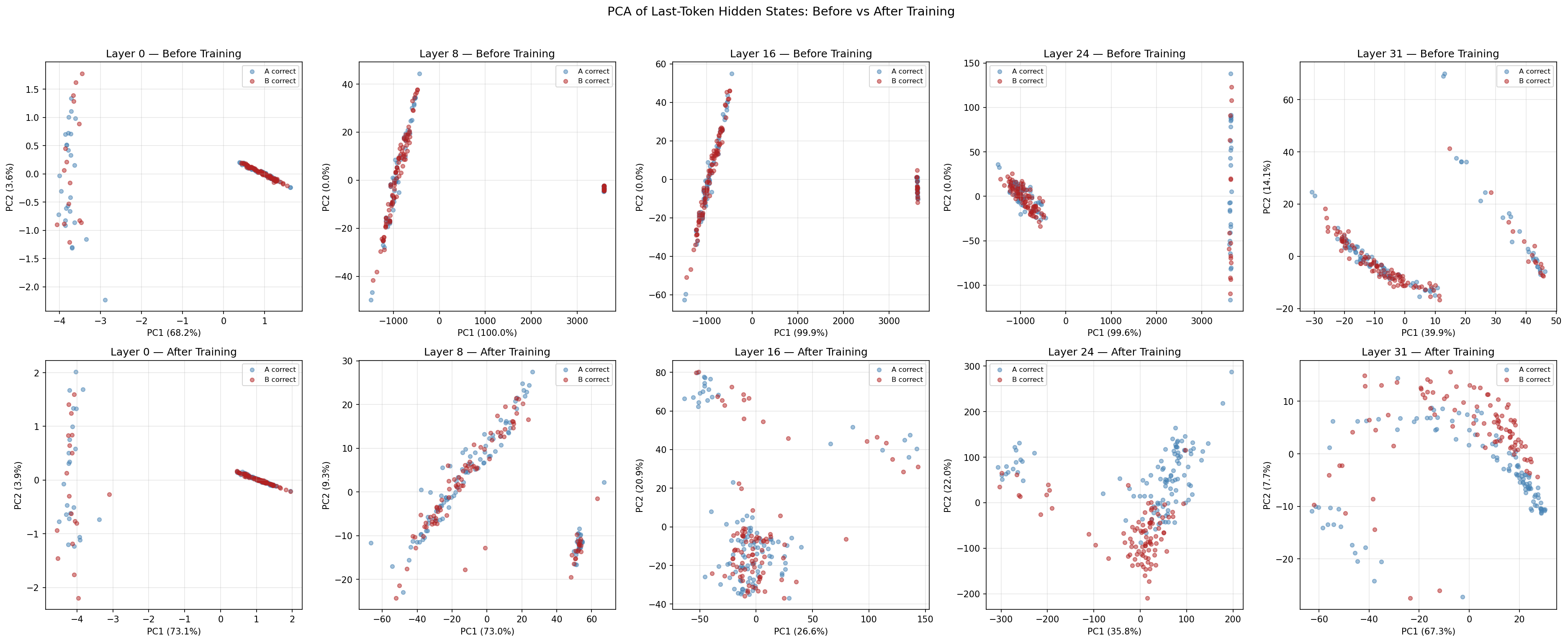
I ran a simple logistic regression on the hidden states at each layer, before and after training. The question was: at which layer can a linear classifier separate “A is correct” from “B is correct”?
What this does: Fit a logistic regression on hidden states from each layer to test how linearly separable the two classes are.
from sklearn.linear_model import LogisticRegression
from sklearn.model_selection import cross_val_score

for layer_idx in [0, 8, 16, 24, 31]:
    clf = LogisticRegression(max_iter=1000)
    scores = cross_val_score(clf, hidden_states[layer_idx], labels, cv=5)
    print(f"Layer {layer_idx}: {scores.mean():.3f}")
The results split the network in half. Layers 0 and 8 showed no improvement, their linear probe accuracy actually decreased slightly (0.545 → 0.490 and 0.500 → 0.475). But layer 16 jumped from 0.455 to 0.825. Layer 24: 0.440 to 0.825. Layer 31: 0.480 to 0.840.
The layers that changed the most (layers 0-1, gradient norm 200+) produced representations that were LESS separable after training. The layers that barely changed (layers 16-31, gradient norm under 2) produced representations that went from random to 84% linearly separable.
Part 5: The Ablation That Broke My Theory
I ran one more experiment. I froze different groups of layers and retrained from scratch, each time with 1,000 optimizer steps. If early layers are doing all the work (that’s what the gradient norms said), then freezing them should destroy performance. Right?
Wrong. Again.
Only late layers trainable (20-31): 67.75%. Only early+middle trainable (0-19): 69.75%. All layers (control): 83.0%. But here’s the one that made me stare at the screen: only middle layers trainable (10-19), with just 10 out of 32 layers unfrozen, hit 84.25%. Nearly matching the main training’s 87.3%.
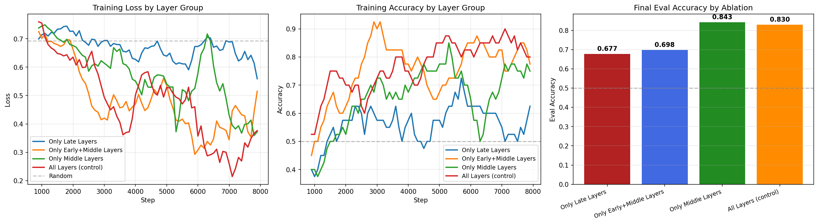
The middle layers alone are almost sufficient. And adding the early layers to them (the “early+middle” condition) actually made things worse — 69.75% versus 84.25%. The early layers, despite receiving 200x more gradient signal in the main training, appear to be destabilizing the representations when trained. They change aggressively, and that aggression interferes with the middle layers’ ability to build useful rankings.
This is a finding I didn’t expect at any point during this experiment. The layers that receive the most gradient signal aren’t just “not the most important” — they’re actively harmful when trained in isolation with the middle layers. The optimal strategy appears to be: let the middle layers learn, and leave everything else alone.
Summary
In this post, I fine-tuned a Phi-3 Mini (3.8B) as a pairwise reranker on MS MARCO using LoRA, and logged per-layer gradient norms, attention patterns, and hidden state linear probes throughout training.
Here’s the thing that ties all of this together. The gradient norms told me where the WEIGHTS changed. The linear probes told me where the REPRESENTATIONS changed. And those are two completely different places.
This reframes how we should think about LoRA fine tuning for ranking. We’re not teaching the model a new concept in its deep layers. We’re not building a “ranking circuit” in the late attention heads. We’re adjusting the input processing, the way tokens are initially encoded and letting the existing transformer stack propagate that adjustment into a useful representation. The ranking knowledge was already distributed throughout the pretrained model. LoRA just adjusted the front door so the right information could flow through.
I ran this experiment on single A100 40GB using 50,000 MS MARCO passage ranking triples.
Did you find this post useful? I am curious to hear from you in comments below.
Comments